Zetaris' virtual pipeline provides a graphical interface for you to transform and prepare your data. Through the pipeline we can expose the end result out in either real-time, or it can be persisted/migrated across into a target system be it a data warehouse or data lake.
There are a number of different functions that the virtual pipeline can use to transform and prepare your data, and the purpose of this guide is to take you through how each of them can be used:
Getting Started with Virtual Pipelines
Getting Started with Virtual Pipelines
The objective here is to build a customer summary by country, showing each customer's number of orders and the lifetime total spend of the customer, aggregating data across multiple data sources and pushing the resultant dataset to a target database (Snowflake in this example).
Start off by invoking the Data Pipeline dialog from the main menu.
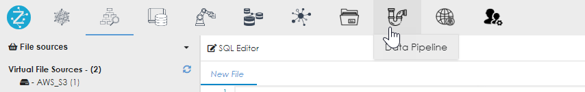
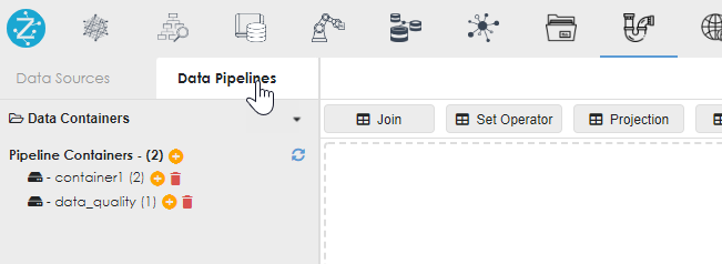
This opens the Data Pipelines dialog, which has 2 main tabs:
|
Data Pipelines Data Sources A pipeline can only exist inside a container. |
 |
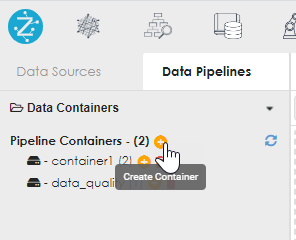 |
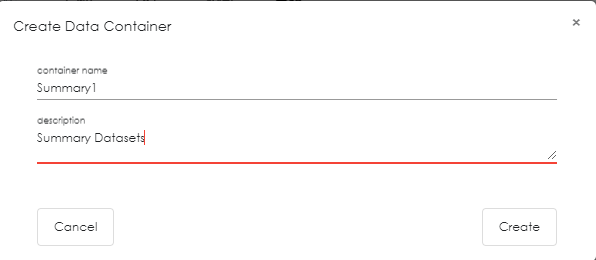
Click the + sign next to containers to add a container. Then appropriately name the container, following the naming rules (no spaces or special characters). |
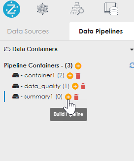 |
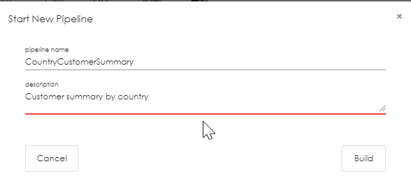
The new container name appears. If it does not, click the refresh icon. Now click the + button to the right of the container name to add / build a new pipeline. Appropriately name the container, following the same naming rules as before. |
 |
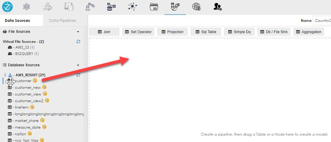
Now click the datasources subtab in the Pipeline dialog to see the sources for the pipeline, as shown below. |
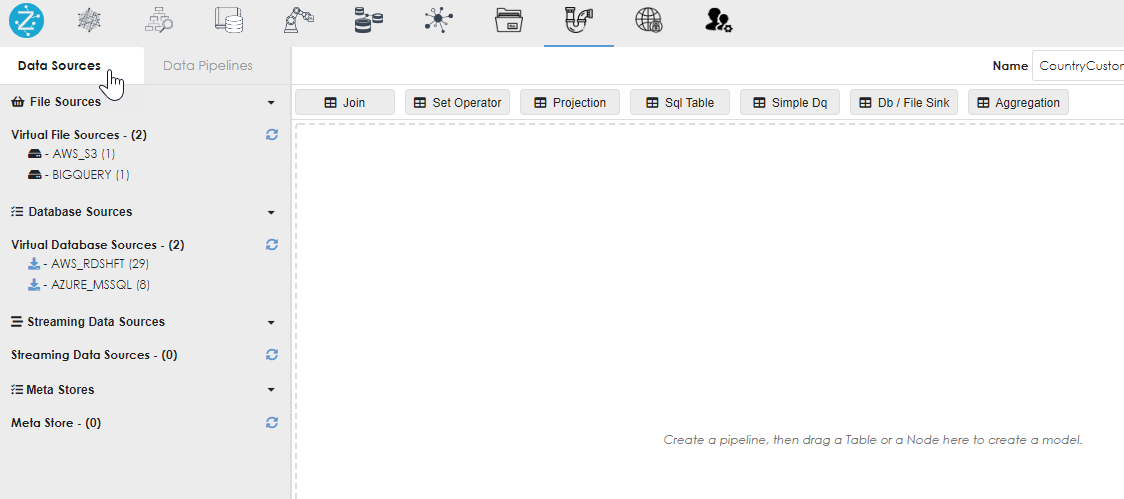
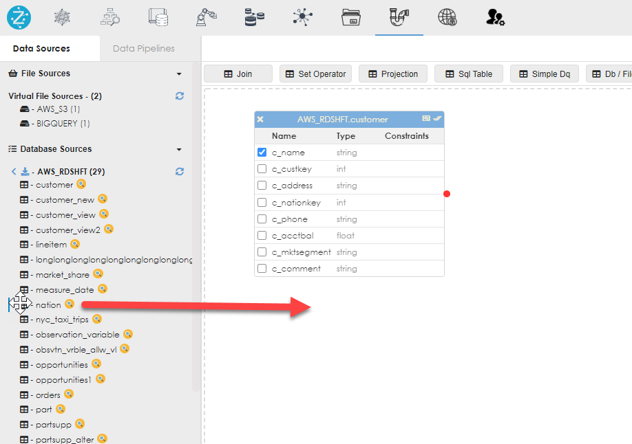
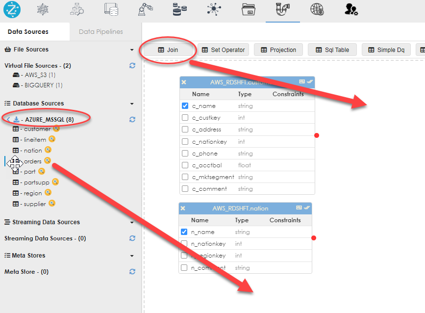
Drag the objects from the data sources into the work area, as shown below. You can drag multiple objects and from different data sources, as shown below.
 |
 |
Join
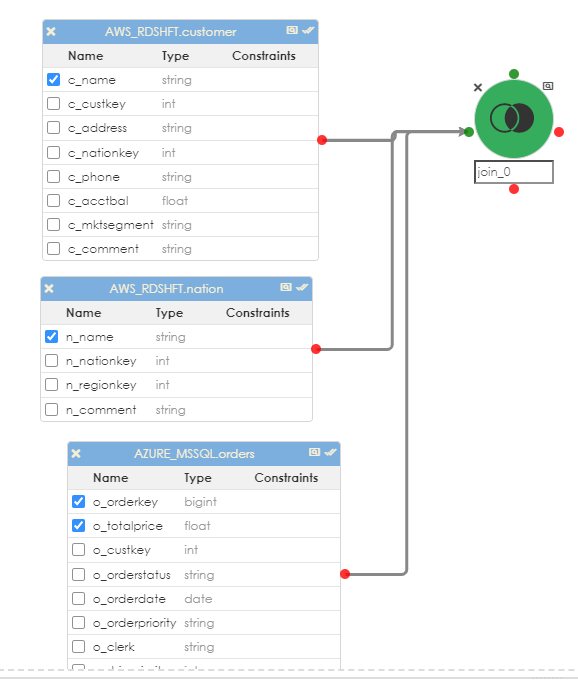
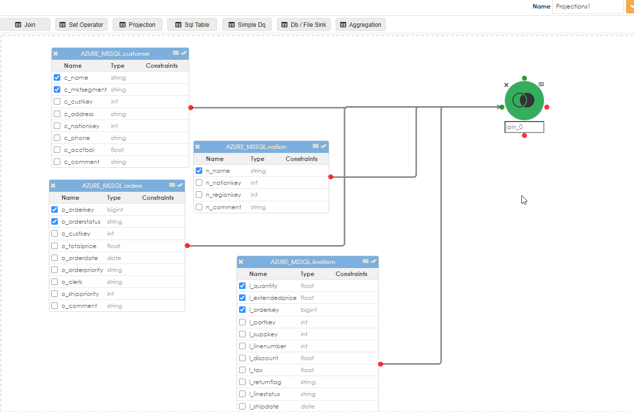
Now you will need to join the objects. Drag the Join operator into the work area as shown below.
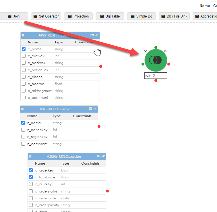
Then link the objects to the join. As shown below, you can link multiple objects to the join and provide a complex join (more than a single condition or relationship). You can optionally name the join object to something that makes sense. Click the checkbox next to the column names that will become part of the pipeline (in most cases, you will not need every column in any given object).
when the join object is clicked, its properties appear in the dialog below, as shown.
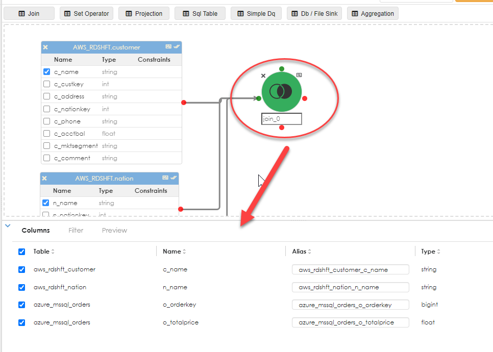
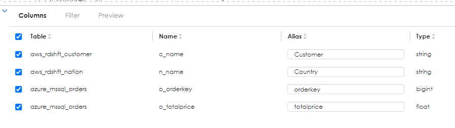
Here you can override the column names with an alias as shown below:
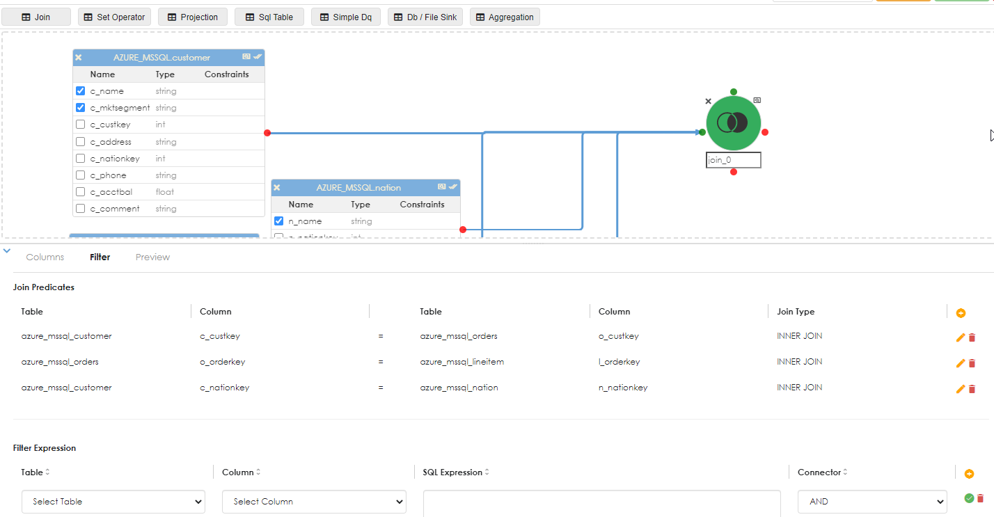
Next, specify the join predicates (conditions) as shown below. Here the Customers table is joined to both the nations table and the orders table.
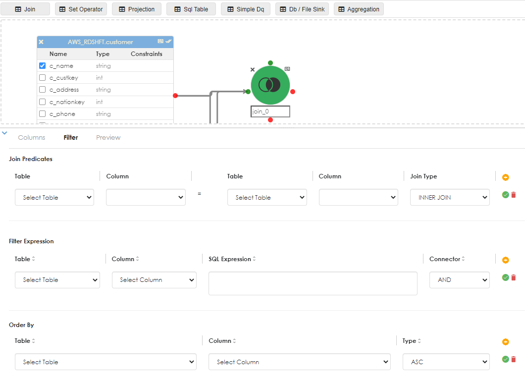
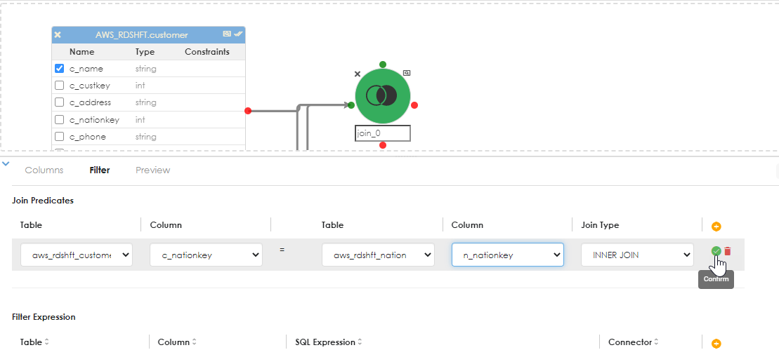
After each step, confirm the join so that saving the object can proceed unencumbered. the columns from the objects will be populated in the dropdown options. Click the Add button in the join predicates sub-dialog to add an additional join condition, as shown below:
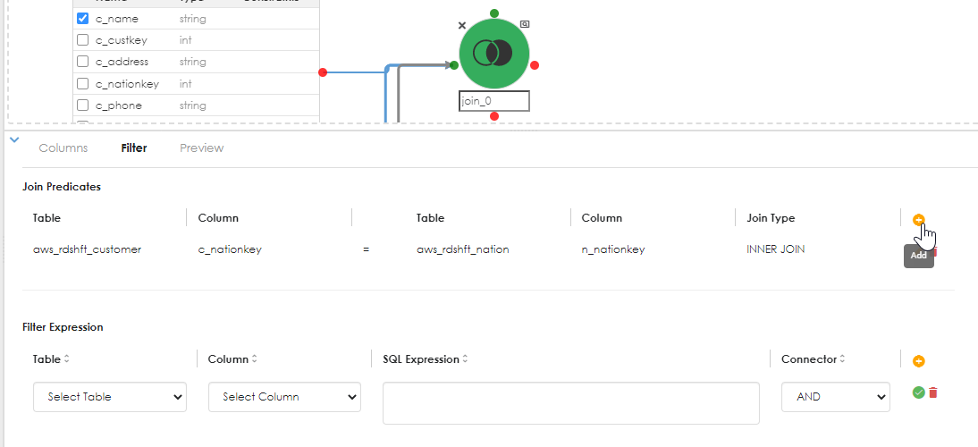
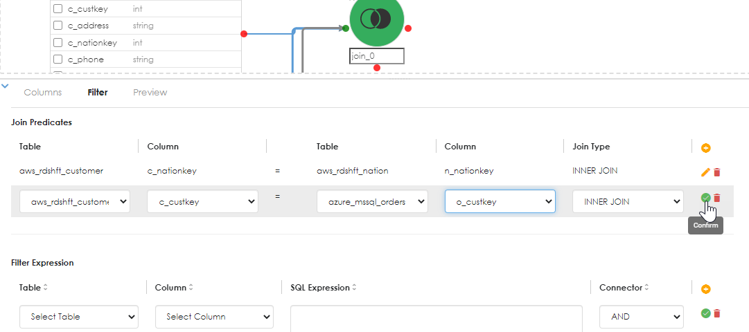
The above shows the second join condition (predicate) added.
Aggregation
You can also apply filters at this point. Once you are done, we can now add an aggregation object, as shown below:
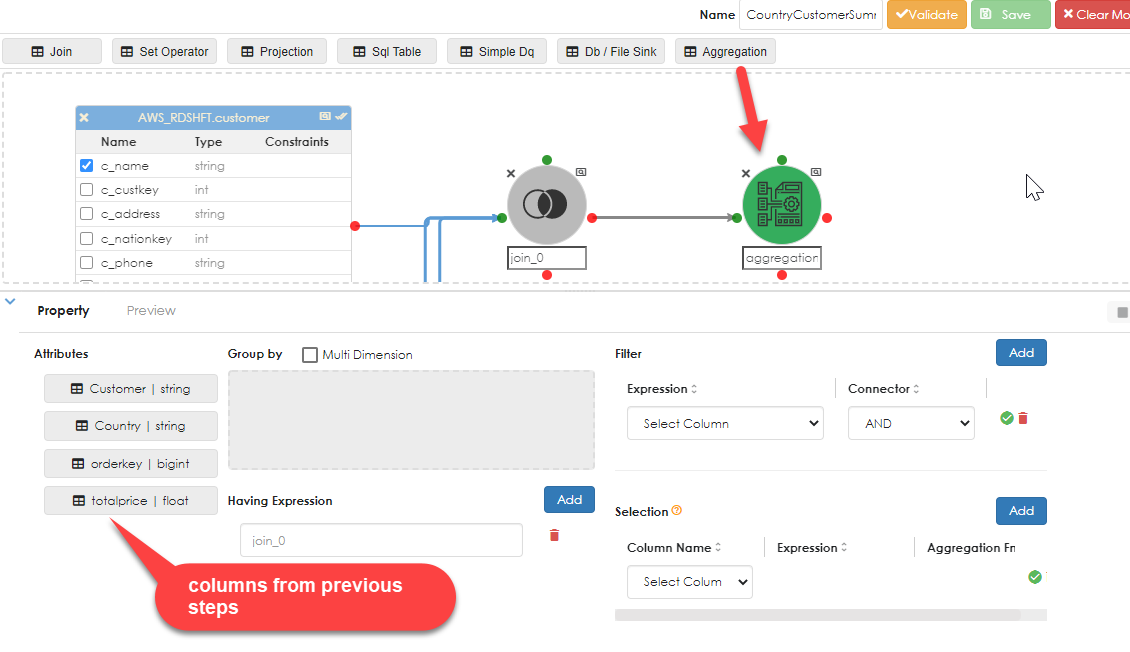
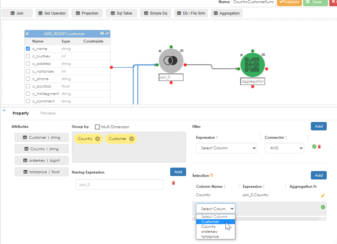
Click the Aggregation object in the work area and the relevant properties dialog opens below, as shown. Drag the dimensions (attributes) for which the aggregation is to be computed into the Group By dialog box. Then it will be time to add the aggregation. Note that in Zetaris a field to be aggregated must be numeric. A count (*) on a non-numeric column is not allowed by the parser.
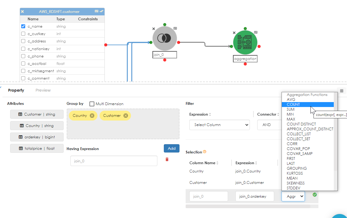
For this example, the number of orders will be counted and the ordertotal will be summed, as shown below:
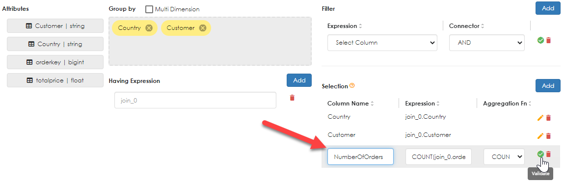
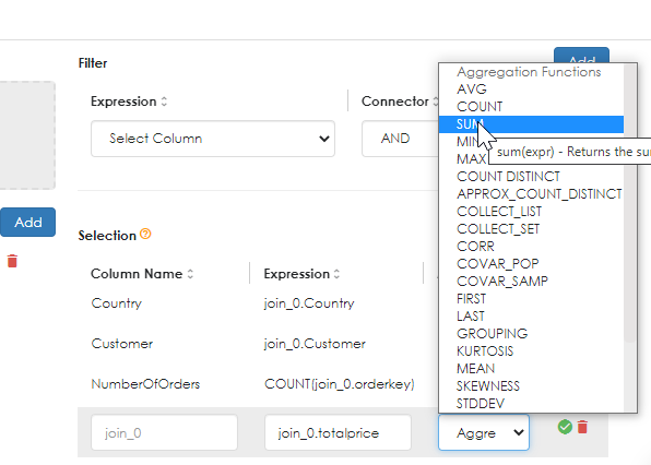
Note how the aggregate expression can be aliased. In the example above, the count of OrderId is aliased as "NumberOfOrders". Do the same again for the TotalPrice, as shown below.
If you want to re-order the selection columns, you will need to delete and start again, paying attention to the order in which you add columns / expressions.
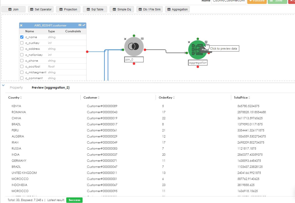
Once this is done, you can now preview the data by clicking the preview symbol of the aggregation object, as shown below:
Db / File Sink
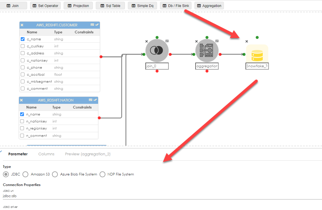
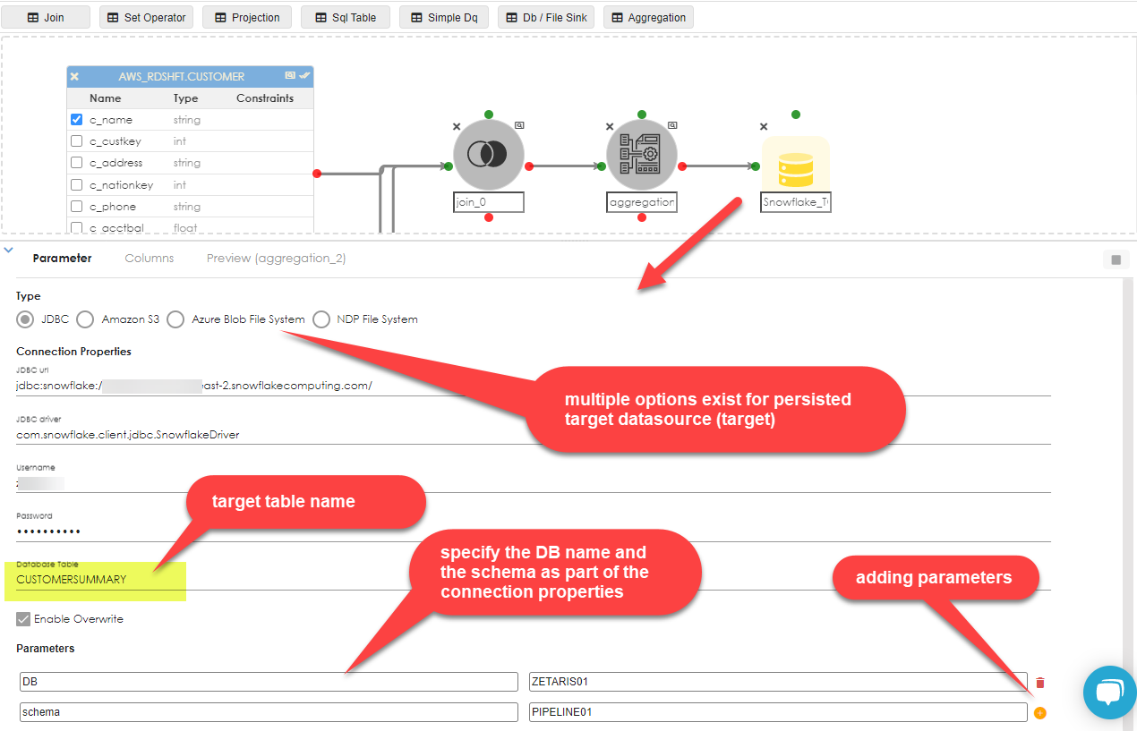
To persist this data into a database source, say Snowflake, drag the Db / File Sink object into the work area and join the Aggregation object to it. Click the sink object as shown below to expose the properties dialg:
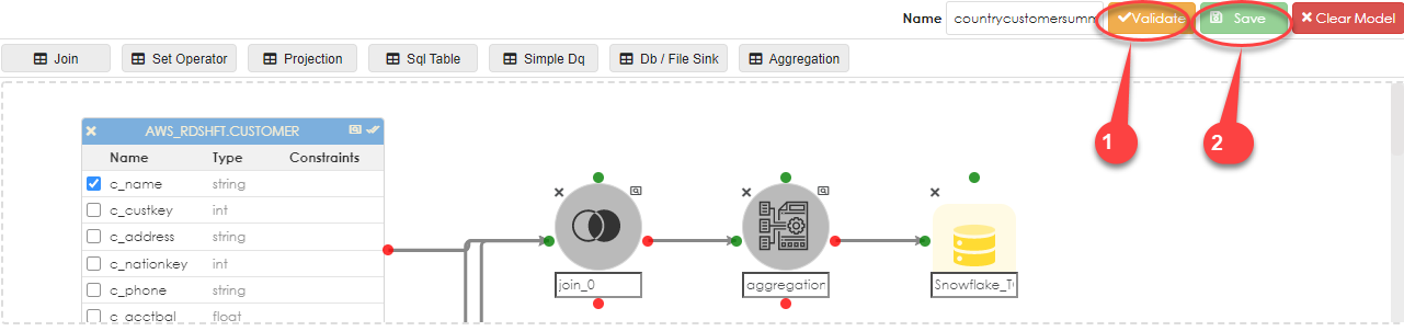 |
Once the properties are configured,validate and save the entire pipeline, so it can be run. |
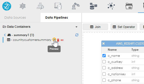
From inside the container, click the preview button to run the pipeline, as shown below:
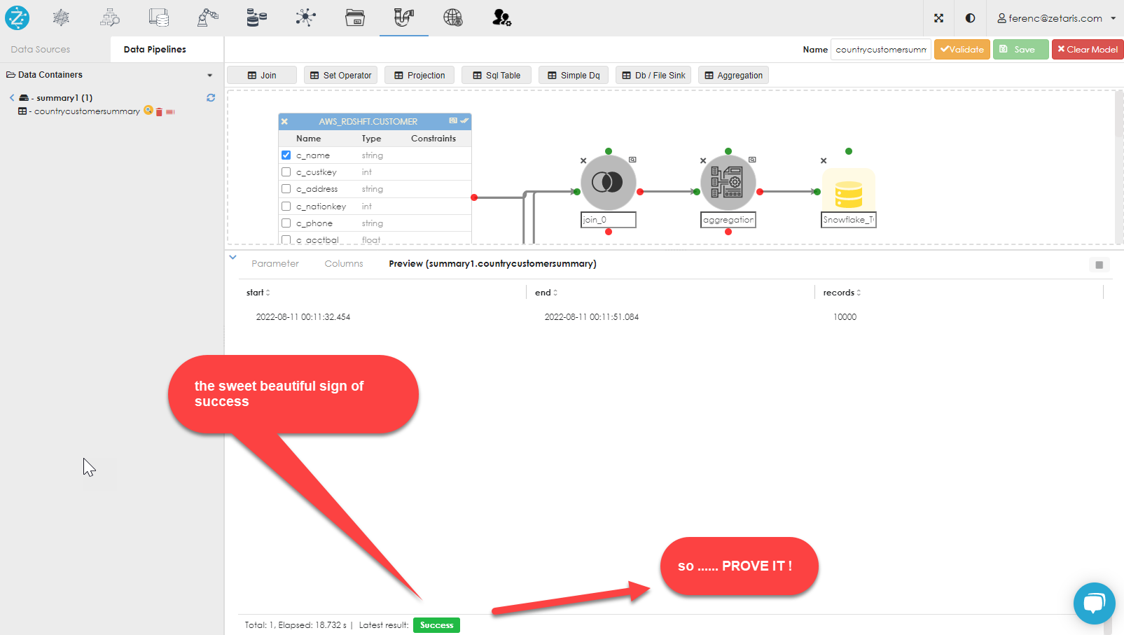
If all goes well, you should see the success indicator in the bottom left of the dialog, as shown below:
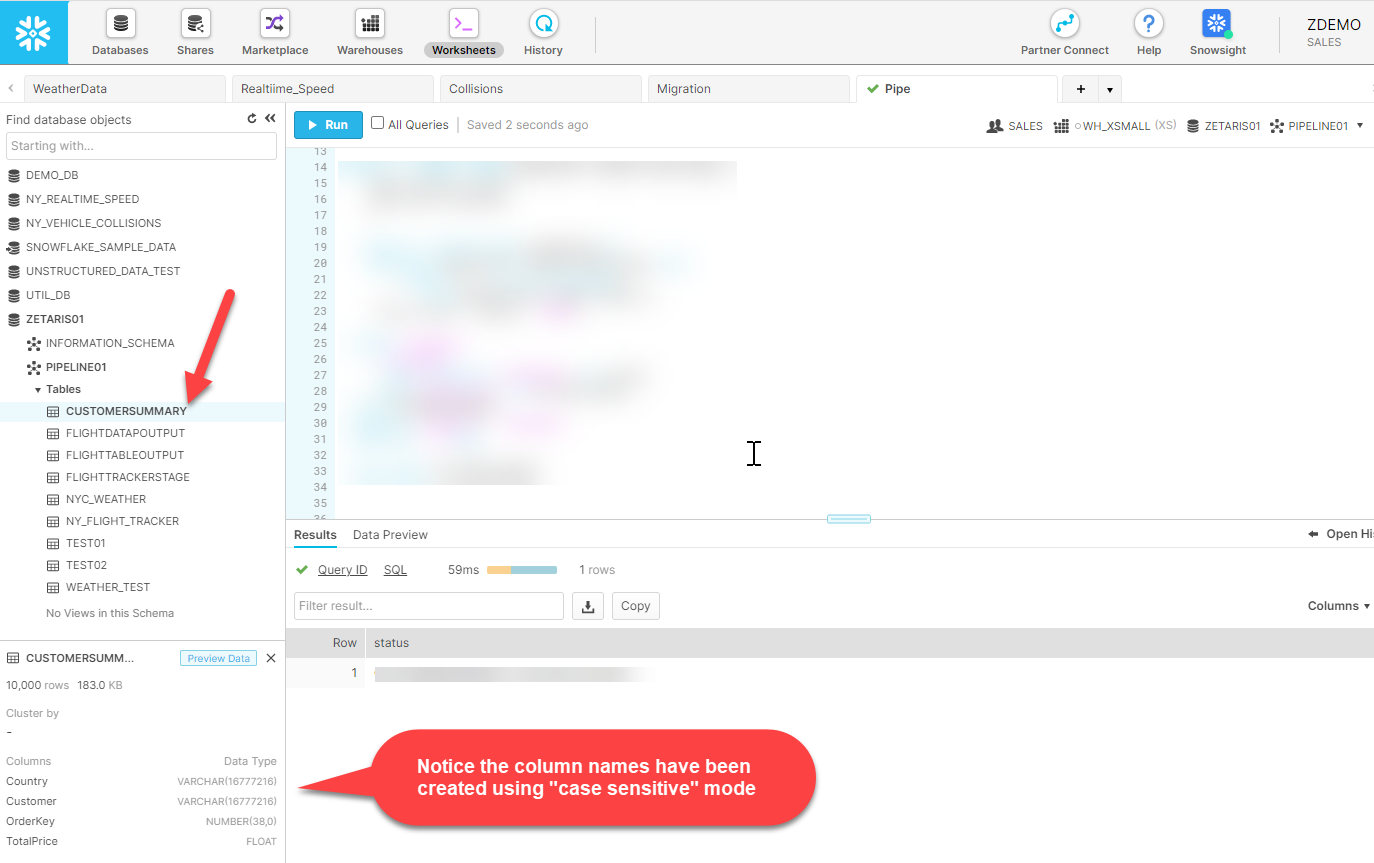
So, here we have the Snowflake environment showing that the table has been created.
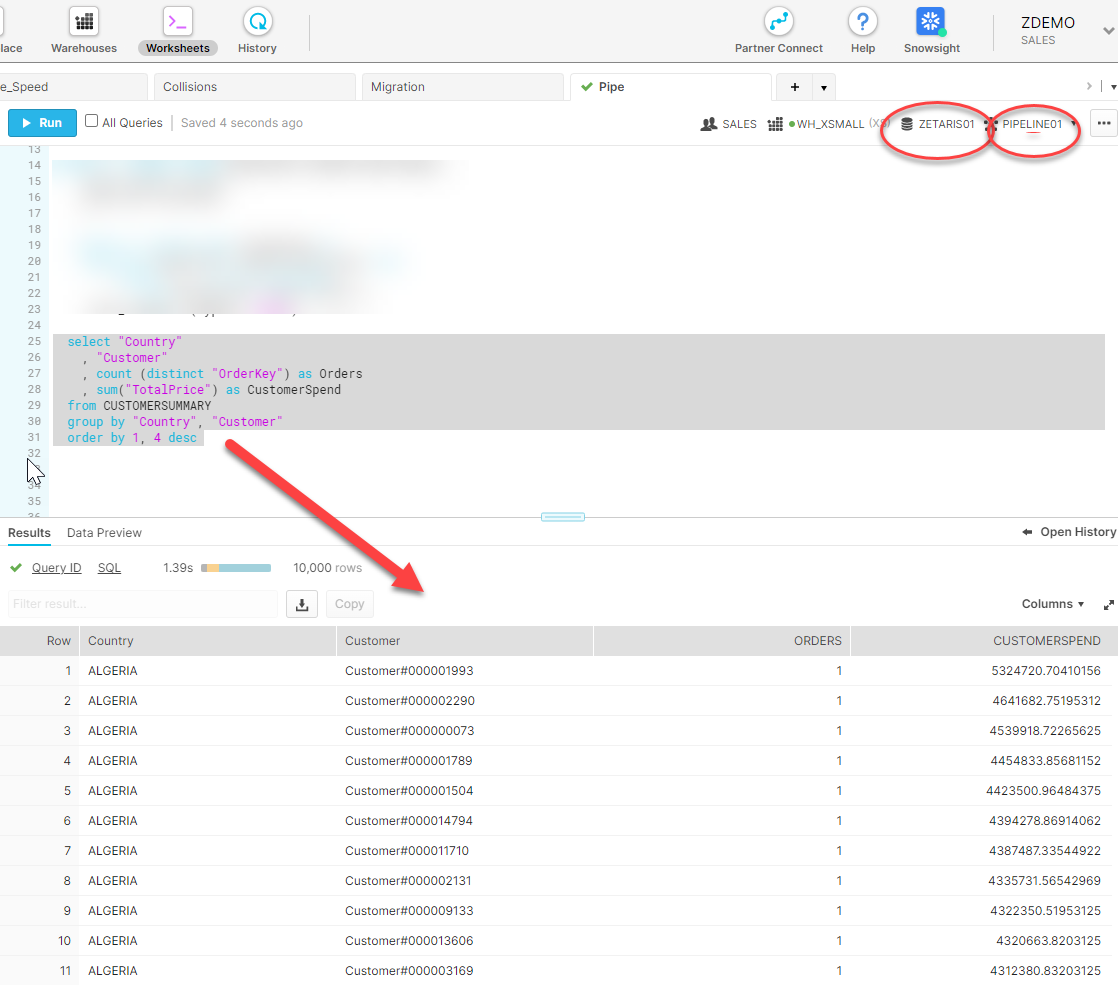
Let's now run a query to prove that the data is in fact present, as shown below:
Projections
Projections in Zetaris pipelines are an intermediary step for processing and manipulating selected data. Below we see a 4 table join, where columns from each of the tables will be selected in the query. The selected columns can be seen where the checkbox exists to the left of the column.
The join details are shown below. 4 tables means there should be at least 3 joins to avoid Cartesian product result sets. Click the validate icon after specifying each join, it is easier to correct mistakes this way than having to debug it later if there are errors.
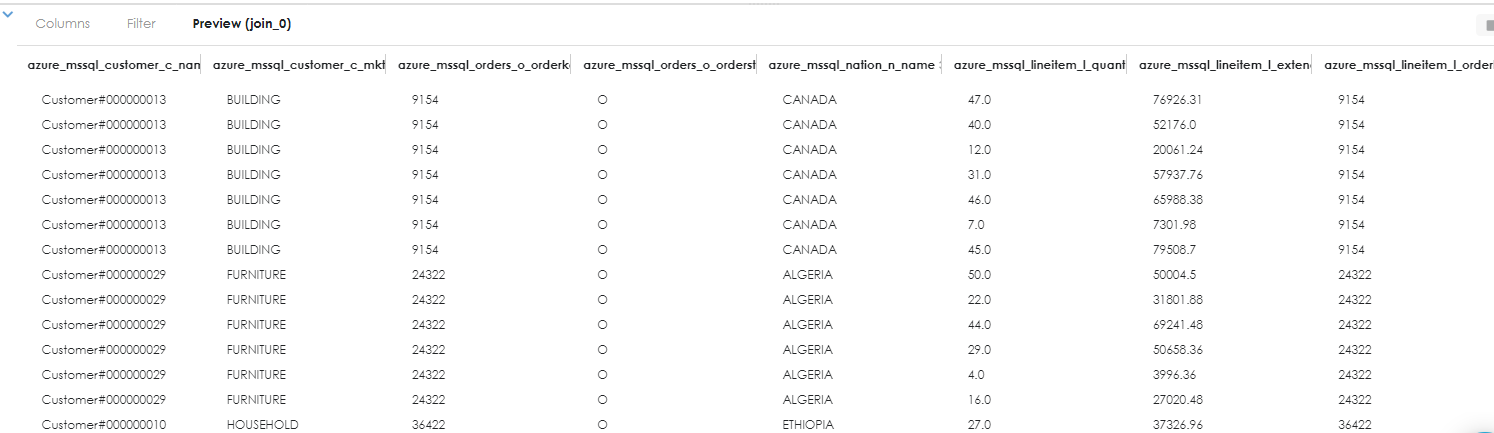
Run a preview on the join to verify it works:
Now drag the projection object and then drag the join to the projection to continue the pipeline processing.
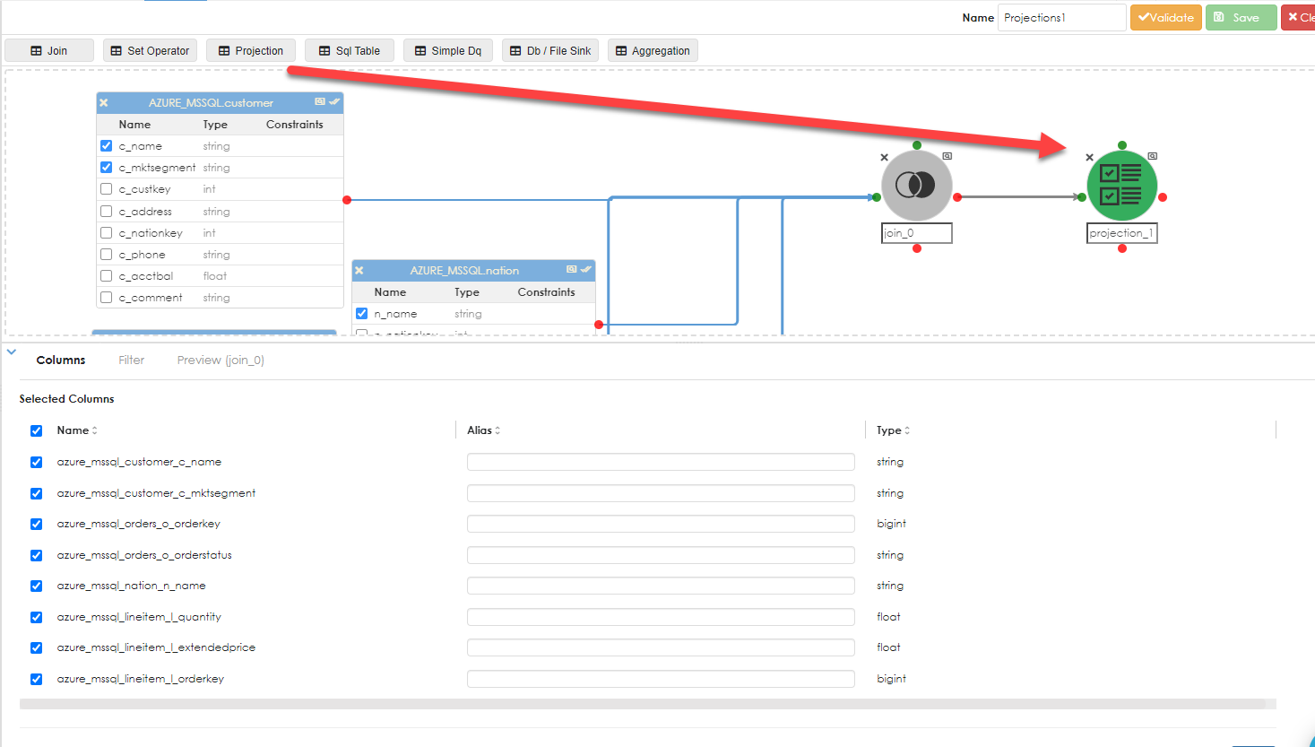
The projection properties dialog opens below. Step 1 in the projection is to rename the columns to something that make sense to the problem being solved or dataset being generated. See below:
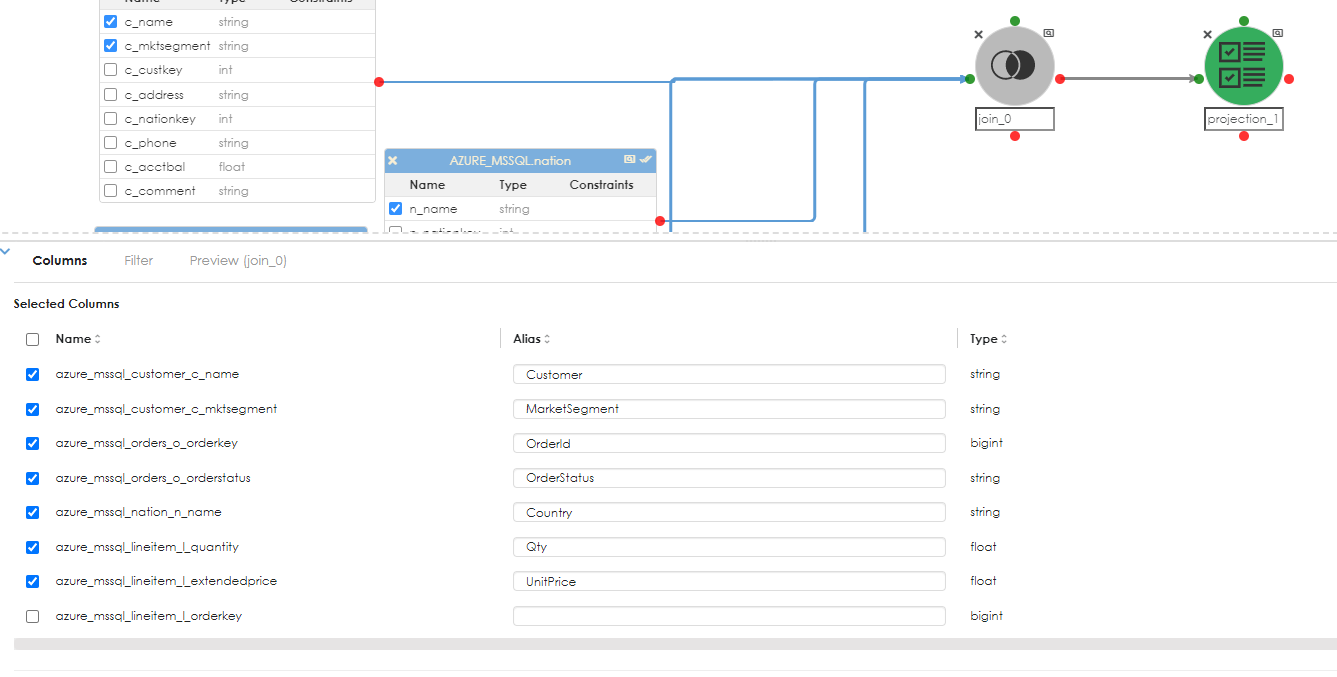
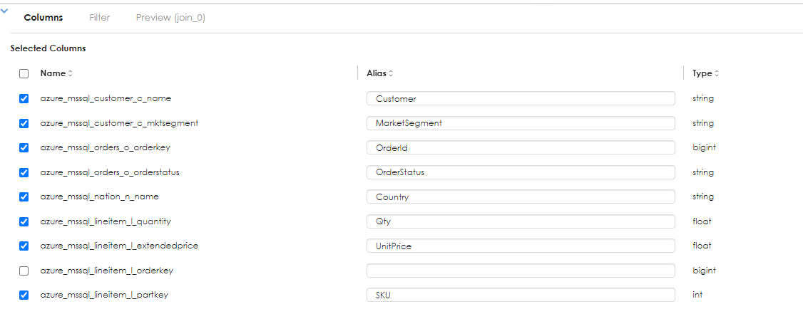
Here the column names have been renamed and where a column is no longer needed in the pipeline, it can be unchecked, as shown above
Another operation that can be performed is to create a computed expression (Virtual column) . The example below shows that for each order line, we can do a simple computation to derive the line total by multiplying the quantity of the orderline, by the product price of the item. in more complex calculations, discount could be applied as a percentage, but for purposes of illustration, this example has been kept simple. Thus:
LineTotal = Quantity * unit Price.
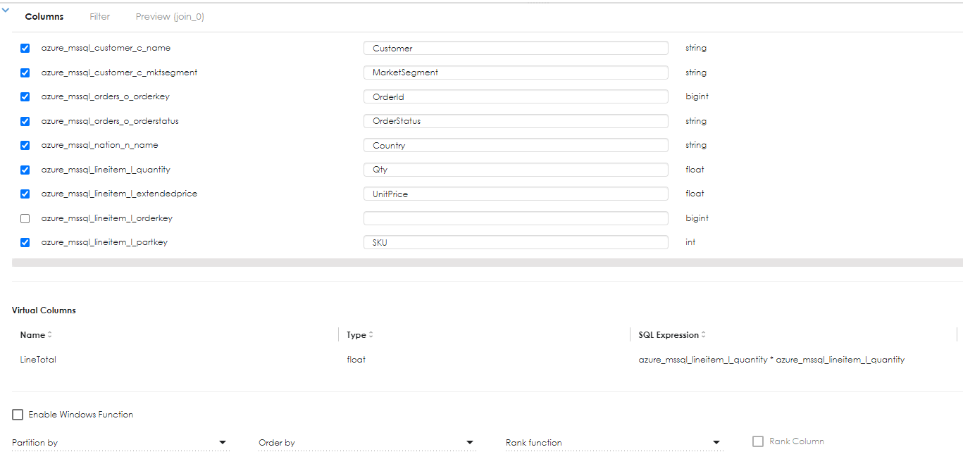
There are other operations available on Projection, such or sorting (Order By) and windowing functions. The screenshot above shows that you can further filter the data sets (filters are also available on joins, where you can restrict the number of rows being returned in a join filter).
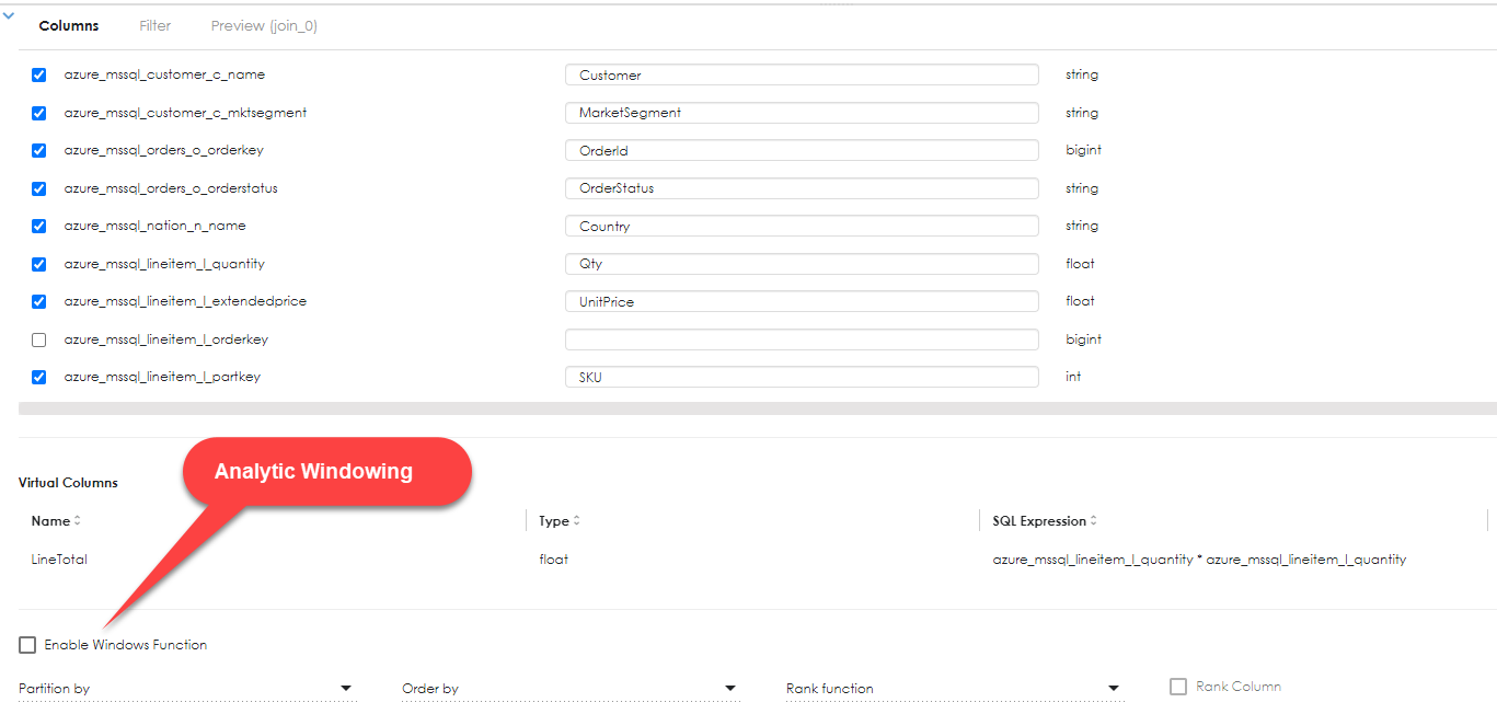
Windowing functions are analytical functions that operate on windowed data sets. If you are unfamiliar with windowing functions, google the term "sql windowing functions", there is plenty of material on the web. Things like ranking, ranking within partitioned data sets, running totals, trailing averages (using LEAD / LAG), Ntile, quartile (statistical functions) are all available.
If you are doing data preparation and needing to invoke windowing functions, it would probably be far easier to do this using a Sql Table, where one can write the SQL exactly as you need it and not need to worry about using a graphical query designer tool. Zetaris pipelines using graphical query designer will be an appropriate solution probably for 90% of the time. The other 10%, where you really want to do things with SQL that would be challenging to parse using a GUI, there is the option of controlling this yourself.
Sql Table
For users of Zetaris who are really comfortable writing SQL, the Sql Table provides the flexibility to write freeform SQL (and that can get pretty ugly sometimes, depending on how and to what level coding standards and best practice is followed) .
Sql Table
There are times when it is just easier to write a SQL statement in freeform. For these occassions, Zetaris provides the Sql Table object. Keep in mind that any SQL functions will be Spark-specific, so if your source environment is Oracle, Sql Server or some datasource that has its own extensions to ANSI SQL, this will not work.
Examples of RDBMS specific SQL extensions
| Source | SQL Extension |
| Oracle | DECODE, INSTR, MOD, "connect by prior parent" |
| Sql Server | convert: convert(<dateime>,112), etc. "For XML", graph QL, etc. |
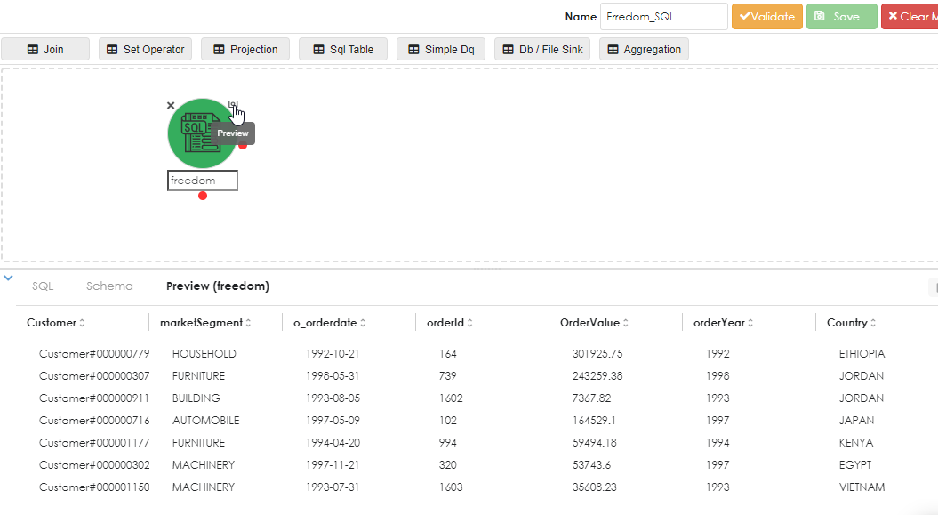
Start off by dragging the Sql Table object into the work area. This will then open an editor in the object proiperties.
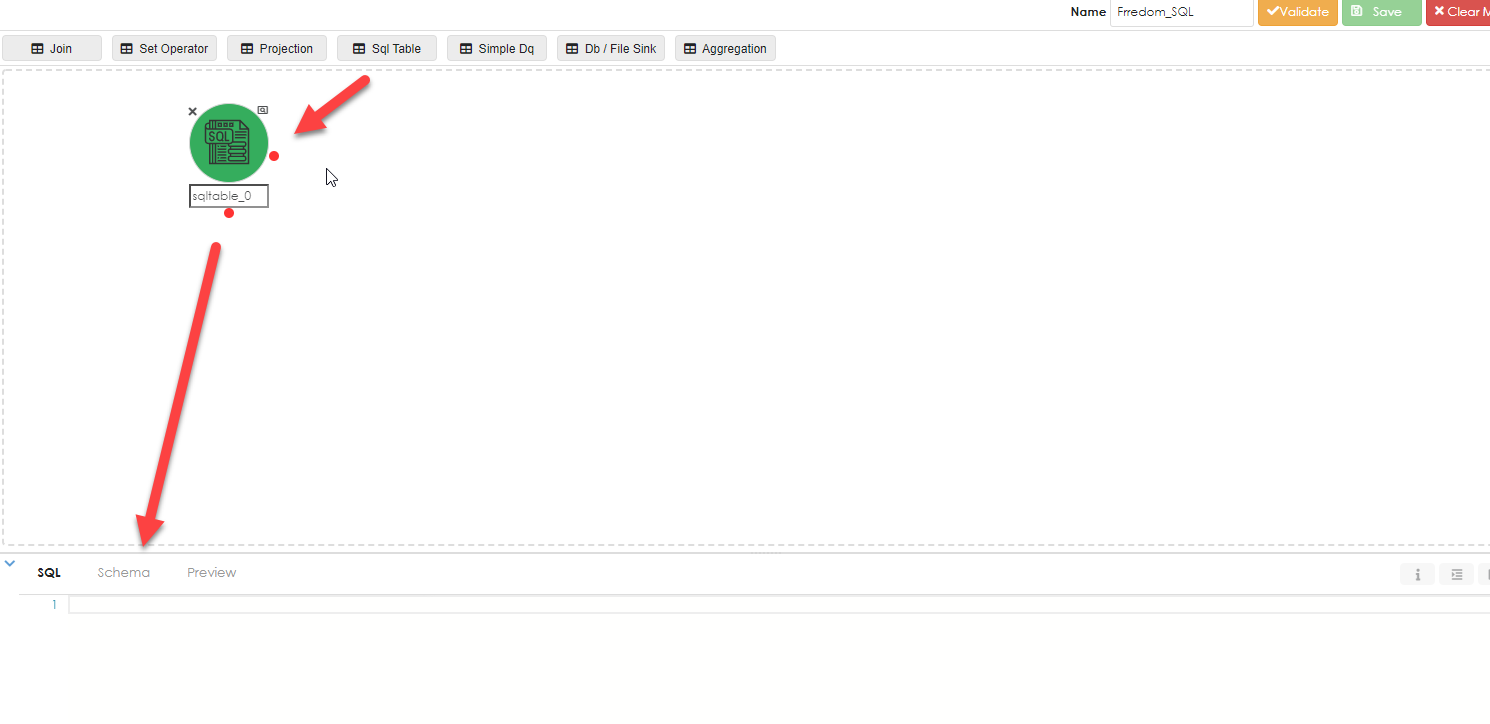
Once you have written the SQL then you will need to click the infer button, as shown below:
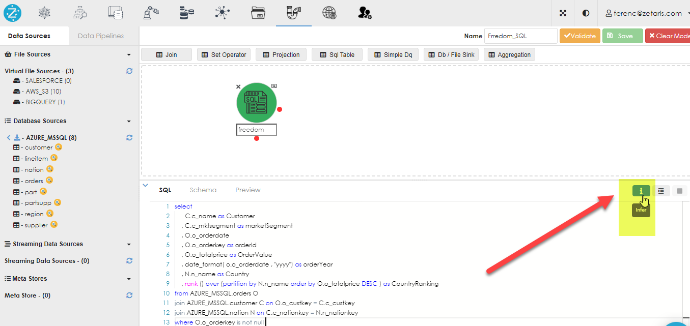
The SQL above reads as follows:
select
  C.c_name as Customer

, C.c_mktsegment as marketSegment

, O.o_orderdate

, O.o_orderkey as orderId

, O.o_totalprice as OrderValue

, date_format( o.o_orderdate , "yyyy") as orderYear

, N.n_name as Country

, rank () over (partition by N.n_name order by O.o_totalprice DESC ) as CountryRanking

from AZURE_MSSQL.orders O

join AZURE_MSSQL.customer C on O.o_custkey = C.c_custkey

join AZURE_MSSQL.nation N on C.c_nationkey = N.n_nationkey

where O.o_orderkey is not null
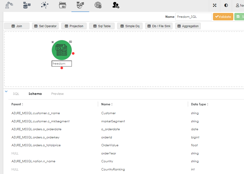
Once you click the infer button, it will generate the query metadata and display it in the Schema subtab of the properties dialog, as below:
Now run the SQL to ensure it works. You can do this by clicking the preview property of the Sql Table object inthe work area.